Coefficient complexity, sensors and noise

This experiment compares coefficient degrees 0–3 for −u″ + q(x; θ) u³ = 1, with zero boundary values, the full prior [0,1000]^(d+1), and target θ₀. Data are generated at θ = 500·1 and rounded to twelve decimal places. The generating parameter is certified against those rounded data before searching. Sensors are uniformly spaced in (0,1).

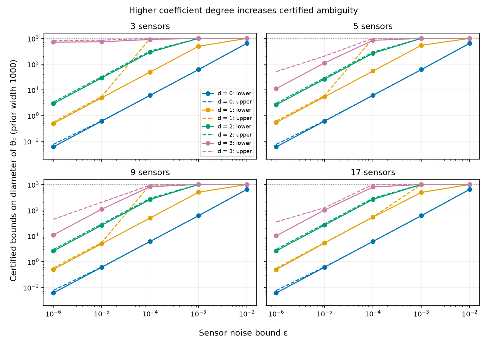
All 80 cells were completed: 4 degrees × 4 sensor counts (3, 5, 9, 17) × 5 noise levels (10⁻² through 10⁻⁶). Every saved pair and paving was replayed with the exact checker. Measured generation and replay time was about 195 seconds on the development machine; this is a timing observation, not a portable bound.

Results at 17 sensors

The entries below are certified lower bounds on the target diameter, with six decimal places retained exactly. Degree-zero upper bounds follow separately.

Degree	ε = 10⁻²	ε = 10⁻³	ε = 10⁻⁴	ε = 10⁻⁵	ε = 10⁻⁶
0	576.108163	55.296296	5.527362	0.552732	0.055272
1	1000	458.982538	45.769866	4.576858	0.457686
2	1000	1000	239.822415	23.980313	2.398029
3	1000	1000	761.827345	85.588919	8.558871

For degree zero, full-prior affine SIVIA proves upper bounds 5295125/8192, 1006875/16384, 50375/8192, 5125/8192, and 625/8192, respectively. Thus at ε = 10⁻⁶, the diameter lies between 0.055272 and 0.076294 (upper rounded outward). The same degree-zero bounds occur at all four sensor counts: each layout includes the central sensor, which dominates this scalar experiment. This supplies a quantitative recoverability baseline under the constant-coefficient model.

At degree three and the same 17 sensors and noise, the certified diameter is at least 8.558871. At noise 10⁻³ or larger, degrees two and three already admit pairs spanning the full prior width, so the diameter is exactly 1000. At only 3 sensors, the cubic model still has certified diameter at least 715.244548 at noise 10⁻⁶. This is a finite-noise result, not an exact-data nonuniqueness theorem. Smaller lower bounds found with more sensors do not prove identifiability. In the original sweep, degrees 1–3 had only the prior-width upper bound 1000. The figure now incorporates tighter follow-up certificates below.

Reproduce and interpret

PYTHONPATH=. python studies/phase_diagram.py
MPLCONFIGDIR=/tmp/twindex-mpl PYTHONPATH=. python studies/phase_figure.py

The search uses three deterministic starts per cell: the generating parameter and two pseudorandom perturbations (seed 20261107 + degree). Of 240 attempted starts, 180 produced certified pairs. Rejected starts include numerical infeasibility and failure to certify the endpoints; certified_starts records successes rather than treating a failed search as evidence. The largest exact-certified gap is retained. Every endpoint also meets ρ/8 ≤ ε/10. The local search has no global optimality guarantee.

The solver order is 24, the exact replay depth is 4, and degree-zero pavings use at most 128 leaves with minimum split width 1/100. The plain/affine checker retains every undecided leaf in the outer enclosure. No local prior restriction is used. The runner checkpoints summary.csv after each cell and stops between cells after a default 28-minute budget; a partial run is not the complete grid.

Exact CSV values and all 100 certificates are in studies/results/phase/. Six representative certificates are copied to examples/study/phase/ and replayed in CI, including both degree-zero noise extremes and the corresponding cubic pairs at 17 sensors. The figure shows the strongest saved certified lower bound (pairs or inside-paving claims) and the smallest saved upper claim as solid and dashed curves, respectively, for every degree. Its dotted line is the prior width. It reads exact claims from certificate files, using CSVs only to locate completed evidence, and matches the entire Problem before combining bounds. This includes affine, monotone and oriented pavings, the original and LP-seeded pairs, and the matching intermediate-degree robustness problems. Rendering uses previously replayed evidence; it does not repeat the expensive exact study replays. An oriented JSON without a checkpointed CSV row is ignored. Finite-budget upper curves can be nonmonotone in noise: a loose result at small noise does not contradict a tighter result on a different, larger-noise problem. Segments connect sampled cells; no bounds between sampled noise levels are asserted.

Monotone full-prior follow-up

The monotone theorem encloses each box using its lower and upper corner solutions. sivia(..., mode="monotone") caches candidates by their exact corner parameter vector and shares identical polynomials in the certificate table. mode="auto" selects this method when the source and boundary hypotheses are proved, falling back to affine bounds otherwise. Explicit monotone mode raises an error when its hypotheses are not proved. Candidate errors retain unresolved boxes. A numerical screen can skip expensive work, but every inside or outside label still requires a VALID exact check, and the final paving is replayed.

With degree three, 17 sensors, and the full prior [0,1000]^4, the first runs (n = 16, depth = 4) gave:

ε	Leaf budget	Outside	Unresolved	Certified upper
10⁻⁴	1024	461	563	1000
10⁻⁵	1024	497	527	1000
10⁻⁶	1024	504	520	1000
10⁻⁵	10000 (width priority)	5606	4394	1000
10⁻⁵	10000 (boundary priority)	9401	599	718.75

There were no inside leaves. The strong lower bounds in the previous table come from separate pair certificates for the identical problem instances. The boundary-priority run proves the first tighter cubic full-prior upper bound: 85.588919 ≤ D ≤ 718.75 at 17 sensors and ε = 10⁻⁵. A later LP-seeded twin search (below) raises the lower side, giving 101.69308 ≤ D ≤ 718.75 on the identical problem. The lower and upper certificates contain exactly identical Problem objects; no local-prior restriction or change to the measured data is involved.

At 10,000 leaves, width-priority generation took about 166 seconds (including its internal exact replay); an additional independent replay took about 69 seconds. Boundary priority took about 267 seconds for generation and 119 seconds for independent replay. Thus the tighter upper bound is achieved by changing the allocation of subdivisions, at a higher verification cost. The upper bound still exceeds the certified pair gap substantially. No claim of a tight diameter, global search optimality, or exact-data identifiability follows.

Reproduce the small runs and the larger width-priority run with:

PYTHONPATH=. python studies/monotone_sweep.py --budgets 1024
PYTHONPATH=. python studies/monotone_sweep.py --budgets 10000 --noise 1/100000 \
  --output studies/results/monotone/large
PYTHONPATH=. python studies/monotone_sweep.py --budgets 10000 --noise 1/100000 \
  --priority boundary --output studies/results/monotone/boundary

The large certificates are repository artifacts under studies/results/monotone/, excluded from the sdist and routine CI replay. The --priority boundary variant processes boxes nearest the prior's target endpoints first; the default --priority width processes the widest target projections first. Both retain complete coverage and recheck every labelled leaf. Neither guarantees that a fixed budget will find tight diameter bounds.

Linearised baseline and LP-seeded twins

studies/linearized_baseline.py linearises the forward map at the generating parameter and solves two linear programs for the range of θ₀. The resulting width D_lin is an uncertified prediction. It lies inside the original pair-lower/paving-upper intervals in all 80 cells (studies/results/phase/linearized_baseline.csv). This comparison uses the pair lower bounds recorded in that baseline table. It does not hold for every stronger lower claim now plotted: the degree-zero inside-paving lower bounds at ε = 10⁻² and 10⁻³ exceed D_lin at all four sensor counts. A local linearisation need not predict the nonlinear diameter exactly.

studies/lp_seeded_pairs.py seeds the exact twin search with the LP optimisers, shrunk by a factor of 0.9 and rounded to rationals, then certifies each twin exactly. It improves 47 of the 80 cells, and every certified lower bound reaches at least 0.8999 D_lin (the 0.9 target less rational rounding) (studies/results/phase/lp_seeded.csv, certificates in studies/results/phase/lp_seeded/). Nothing in either script is trusted: every bound reported comes from an exact VALID check.

Robustness and intermediate-degree outer bounds

The follow-up in studies/robustness.py keeps the full prior and target θ₀ throughout. Every reported interval combines an LP-seeded pair with a monotone boundary-priority paving for the identical Problem, including its rounded data. All 16 cases use 1,024 leaves, numerical order 16 and exact depth 4 for the paving, with independent exact replay. The pair proposals use order 48 and margins 0.9, 0.7, 0.5, 0.3 and 0.1; only certified endpoints are retained. These are finite-budget enclosures, with no optimality claim.

For cubic coefficients, three off-centre generators use 17 uniform sensors: (200,800,300,700), (800,200,700,300), and (232,729,262,650). The last is an integer draw from [100,900] using NumPy seed 20261107. This checks three additional synthetic instances; it is not a statistical robustness guarantee.

At θ = 500·1, the nine-sensor comparison uses exactly these rational layouts:

• Centre: 0.42, 0.44, …, 0.58.
• Boundary: 0.02, 0.04, 0.06, 0.08, 0.50, 0.92, 0.94, 0.96, 0.98.
• Uniform control: 0.1, 0.2, …, 0.9.

The boundary layout includes one central sensor; all three layouts are symmetric and have nine distinct sensors. Data are generated separately at each layout and rounded to twelve decimal places. Thus these are controlled synthetic sensor-design comparisons, not certificates about a shared measured dataset. Different certified lower bounds alone do not prove an ordering of the true diameters when their certified intervals overlap.

At 1,024 leaves, all entries below are exact terminating decimals:

Case	ε	Certified lower	Certified upper
alternating	0.0001	708.1963	1000
alternating	0.00001	102.76349	1000
reversed	0.0001	702.924157	1000
reversed	0.00001	100.584831	1000
random	0.0001	727.555605	1000
random	0.00001	99.111121	1000
centre	0.0001	1000	1000
centre	0.00001	883.674355	1000
boundary	0.0001	927.710191	1000
boundary	0.00001	667.107811	1000
uniform9	0.0001	819.821345	1000
uniform9	0.00001	109.515713	1000
degree1	0.0001	49.017	54.595947265625
degree1	0.00001	4.9017	5.5694580078125
degree2	0.0001	263.064973	500
degree2	0.00001	26.306498	218.75

The intermediate-degree upper bounds improve with budget:

Degree	ε	U at 128 leaves	U at 1,024 leaves
1	0.0001	60.546875	54.595947265625
1	0.00001	7.8125	5.5694580078125
2	0.0001	875	500
2	0.00001	750	218.75

The lower column above records the pair gap consistently. The degree-one pavings also contain inside leaves and therefore certify stronger lower bounds themselves: 222375/4096 = 54.290771484375 at ε = 10⁻⁴, and 43625/8192 = 5.3253173828125 at ε = 10⁻⁵. Combining their inner and outer claims gives 54.290771484375 ≤ D ≤ 54.595947265625 and 5.3253173828125 ≤ D ≤ 5.5694580078125, respectively. All other baseline pavings in this follow-up have no inside leaves. In particular, absence of inside boxes does not imply absence of compatible points: the separate pairs establish nonemptiness.

A larger, 10,000-leaf uniform-nine-sensor run at ε = 10⁻⁴ proves 819.821345 ≤ D ≤ 937.5. In contrast, the centre-clustered layout has D = 1000 at the same noise and generating parameter. The disjoint certified intervals establish a strict sensor-layout comparison for these synthetic instances. This is stronger than comparing two lower bounds. The uniform run has 9,037 outside and 963 unresolved leaves, no inside leaves; retaining all unresolved leaves is essential to the outer bound. At 1,024 leaves its upper bound was still 1000.

The figure below compares the layouts using the best saved pair lower bound and paving upper bound per instance. Endpoint labels are approximate; the CSV and tables give exact rationals or terminating decimals.

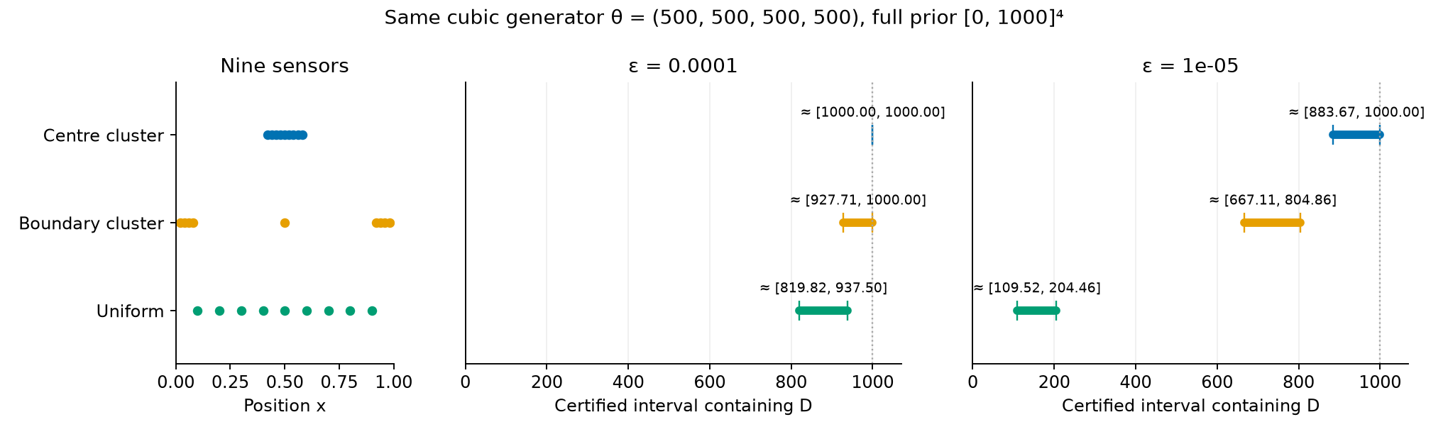
At ε = 10⁻⁵, the 10,000-leaf uniform run similarly proves 109.515713 ≤ D ≤ 718.75, strictly below the centre layout's lower bound 883.674355. It has 9,383 outside and 617 unresolved leaves. Thus the uniform layout has a strictly smaller target diameter than the centre layout at both tested noise levels. The boundary layout's interval overlaps the others, so these experiments do not establish its ordering.

Reproduce the follow-up and figure with the studies extra installed:

PYTHONPATH=. python studies/robustness.py --max-leaves 1024
PYTHONPATH=. python studies/robustness.py --max-leaves 128 \
  --cases degree1 degree2 --output studies/results/robustness/budget128
PYTHONPATH=. python studies/robustness.py --max-leaves 10000 \
  --cases uniform9 --output studies/results/robustness/budget10000
MPLCONFIGDIR=/tmp/twindex-mpl PYTHONPATH=. python studies/robustness_figure.py

All 22 pair/paving combinations (44 certificates) are saved under studies/results/robustness/, with exact CSV summaries and timing fields. Every pair/paving combination was checked to have identical full Problem objects, also across the repeated budgets. Nine smaller certificate copies in examples/study/robustness/ are replayed in CI, including the degree-one inner/outer enclosure and both intermediate-degree 128-leaf pavings. Only the summary CSVs and CI samples enter the source distribution; the larger evidence stays in the repository. The study README records numerical versions and rounding conventions. The overall run stayed within the requested 45-minute compute budget; the 10,000-leaf uniform runs took about 398 and 373 seconds including generation, its internal replay, and an additional exact replay.

Oriented full-prior follow-up

Oriented pavings use θ = o + Aφ with a rational, invertible matrix. The untrusted generator proposes directions using a numerical sensitivity SVD; the checker inverts the rounded matrix exactly and verifies that the root covers the transformed entire prior. Leaves use affine polynomial families in φ. Only the intersection with the original prior needs nonnegative coefficients; a leaf centre may lie outside it. No compatible point is removed by a numerical screen or an undecided leaf.

For the headline cubic problem (17 uniform sensors, ε = 10⁻⁵), a 1,024-leaf paving proves 101.69308 ≤ D ≤ 125.01258, rounding outwards. Its 834 outside and 190 unresolved leaves enclose θ₀ inside [437.33, 562.36]. This uses the identical full Problem as the LP-seeded pair, improving the monotone upper bound 718.75. Generation took about 335 seconds and exact replay about 269 seconds. Smaller budgets or other splitting metrics can give much looser bounds; orientation does not guarantee a tight result for a fixed budget.

Reproduce the headline and the budgeted multi-instance follow-up with:

PYTHONPATH=. python studies/oriented_sivia.py --leaves 1024
PYTHONPATH=. python studies/oriented_sweep.py --leaves 512 --minutes 40

The sweep loads existing pair certificates, preserving their exact data, sensors, model, prior and target. It saves a complete covering tree, then starts a fresh Python process to replay both certificates and require full Problem equality before recording the CSV row. Cases with a certified pair spanning the entire prior are skipped because their diameter is already exactly 1000. The time limit is checked between complete cases, so the final case can overrun it. A partial sweep is reported as partial. Numerical order is 32, candidate degree 14 and exact replay depth 4; split axes use whitened units. Large certificates remain repository-only under studies/results/oriented/.

The degree-two robustness problems are exactly identical to the corresponding 17-sensor phase problems (including rounded data). Their oriented upper bounds therefore apply to both studies. The sensor-layout figure above takes the smallest saved upper bound per instance across monotone and oriented runs. For example, at ε = 10⁻⁴ the 512-leaf oriented uniform run leaves U = 1000, so the existing monotone U = 937.5 remains the reported upper bound. At ε = 10⁻⁵, oriented U < 204.464 versus centre-cluster L > 883.674 proves a diameter separation exceeding a factor of 4.32 for these synthetic designs.

The new boundary-cluster upper bound establishes a stronger conclusion at ε = 10⁻⁵: uniform < boundary cluster < centre cluster in true target diameter. The certified intervals are disjoint: [109.515713, 204.463569], [667.107811, 804.857168], and [883.674355, 1000], respectively (upper endpoints rounded outwards). This compares separately generated, controlled synthetic data for each layout, not three interpretations of one shared measured dataset.

Completed oriented sweep rows

Each row below passed fresh-process exact replay with its matching pair. Upper endpoints are rounded up to six decimal places; the CSV stores the exact rationals. A bound of 1000 is a valid but uninformative upper bound, and does not replace a stronger existing monotone result.

Case	ε	Pair lower	Oriented upper (512 leaves)
uniform9	0.00001	109.515713	204.463569
uniform9	0.0001	819.821345	1000
centre	0.00001	883.674355	1000
degree2	0.00001	26.306498	29.458665
degree2	0.0001	263.064973	292.894912
alternating	0.00001	102.763490	174.434815
reversed	0.00001	100.584831	173.329700
random	0.00001	99.111121	167.172144
boundary	0.00001	667.107811	804.857168
boundary	0.0001	927.710191	1000

This budget-limited follow-up completed 10 pair/paving replays in about 43.6 minutes of generation plus replay. There were no numerical failures or inside leaves. The centre layout at ε = 10⁻⁴ was skipped because its pair already proves D = 1000. The remaining cubic phase cells were not attempted within this budget; the table is not a completed phase-grid sweep. Stronger bounds at larger budgets or with other orientations remain possible.

Oriented phase-grid follow-up

This budgeted follow-up starts with the five requested cubic cells, then considers degree-one and degree-two cells at noise levels 10⁻⁶, 10⁻⁵ and 10⁻⁴. It skips pairs spanning the prior width. Each input is the stronger saved pair (original or LP-seeded), after requiring exact equality of the full Problem. Every row is checkpointed only after a fresh interpreter replays its paving and pair VALID and checks their exact Problem equality and L ≤ U.

All rows use 512 leaves, solver order 32, candidate degree 14 and exact replay depth 4. The following are the completed rows in studies/results/oriented/phase/summary.csv; this is a partial phase-grid sweep. The table reports the pair lower bound rounded down and oriented upper bound rounded up to six decimals. Exact rational claims, leaf counts, evidence paths and timings are in the CSV. The figure takes the best of these and earlier saved certificates, including stronger inside-paving lower claims where present.

Degree	Sensors	ε	Pair lower	Oriented upper
3	17	1/1000000	10.169308	34.961378
3	5	1/100000	111.555584	205.793378
3	5	1/1000000	11.155558	51.172039
3	9	1/100000	109.515713	204.463569
3	9	1/1000000	10.951571	44.143691
1	17	1/1000000	0.490170	0.557429
1	9	1/1000000	0.499796	0.568988
1	5	1/1000000	0.538124	0.613491
1	3	1/1000000	0.493356	0.560212
1	17	1/100000	4.901700	5.460337
1	9	1/100000	4.997952	5.568253
1	5	1/100000	5.381232	5.996331
2	17	1/1000000	2.630650	3.007168
2	9	1/1000000	2.604685	2.981068

Thirteen rows strictly improve the previously best saved upper bound. The cubic nine-sensor result at 10⁻⁵ reproduces the existing robustness bound on the identical Problem. All 80 combined phase-grid enclosures satisfy L ≤ U.

Completed: 14 pair/paving combinations (28 fresh exact certificate replays), about 45.1 minutes of measured generation plus replay. Numerical failures: 0. These are local timing observations, not portable performance guarantees. The time limit is checked between complete cases and may overrun on the final case. Remaining cells are not inferred from missing rows; an uncheckpointed JSON is not a completed result. All unresolved leaves remain in the upper enclosure. No optimality or convergence-rate claim follows from the tighter bounds.

The two degree-two priority cells ran in parallel with the tail of the main sweep, in phase/priority_degree2/. Their subset CSV is retained and their rows are consolidated into the main phase CSV. The summed timings above count overlapping work; they are not elapsed wall time or a controlled benchmark.

PYTHONPATH=. python studies/oriented_sweep.py --phase --leaves 512 --minutes 40 \
  --output studies/results/oriented/phase
PYTHONPATH=. python studies/oriented_sweep.py --phase --leaves 512 --minutes 6 \
  --cases d2_m17_eps1000000 d2_m9_eps1000000 \
  --output studies/results/oriented/phase/priority_degree2
MPLCONFIGDIR=/tmp/twindex-mpl PYTHONPATH=. python studies/phase_figure.py

The runner preserves existing CSV rows and skips completed pair/budget entries when resumed. Larger budgets produce separate certificates and rows. Large JSON artifacts stay in the repository; only the summary CSV enters the sdist.

Final compute round

The final round uses the same resumable runner and exact replay procedure in a separate studies/results/oriented/phase2/ directory. It prioritises degree two with 5 and 3 sensors at ε = 10⁻⁶, then degree one with 3 sensors at ε = 10⁻⁵, before the remaining degree-two and cubic cells. Each input retains the full original Problem, choosing the stronger original or LP-seeded pair. Pairs that already span the full prior width are skipped.

PYTHONPATH=. python studies/oriented_sweep.py --phase-final --leaves 512 --minutes 45 \
  --output studies/results/oriented/phase2
MPLCONFIGDIR=/tmp/twindex-mpl PYTHONPATH=. python studies/phase_figure.py

Resuming this command keeps existing rows and skips their completed pair/budget entries. The figure reads exact certificate claims across both rounds, matched by the entire Problem, and retains an earlier upper bound whenever it is stronger. An uncheckpointed JSON does not contribute a plotted bound.

Completed: 15 cells / 30 fresh VALID certificate replays, with 11 improved upper bounds relative to the earlier best saved claims. The round took about 48.4 minutes of measured generation plus replay. The last cell began before the 45-minute cutoff and completed after it; the limit is checked between complete cells. Numerical failures: 0. Every paving has 512 leaves and no inside leaves. All unresolved leaves are retained. Lower bounds below come from the matching pair, rounded down; upper bounds are rounded up to six decimal places.

Degree	Sensors	ε	Pair lower	Oriented upper
2	5	1/1000000	2.630650	3.007133
2	3	1/1000000	2.908070	3.348415
1	3	1/100000	4.933564	5.494919
2	9	1/100000	26.046847	29.169188
2	5	1/100000	26.306498	29.463499
2	3	1/100000	29.080705	32.510182
2	9	1/10000	260.468472	290.405422
2	5	1/10000	263.064973	293.151431
2	3	1/10000	290.807050	323.740148
3	3	1/1000000	715.244548	832.385177
3	3	1/100000	734.308365	850.134935
3	3	1/10000	908.228493	1000.000000
3	17	1/10000	799.017994	1000.000000
3	9	1/10000	819.821345	1000.000000
3	5	1/10000	839.524336	1000.000000

The four cubic cells at ε = 10⁻⁴ are honest non-improvements: oriented U = 1000 remains uninformative. For nine sensors, the earlier monotone upper bound 937.5 remains the best claim and is retained in the figure. The other three cells retain the prior-width upper bound. The two cubic three-sensor cells at smaller noise improve the upper side, while still certifying substantial ambiguity. All 80 combined exact phase enclosures satisfy L ≤ U. No tighter bounds are inferred at unsampled noise levels, and no optimality claim follows.